Looking at the Environment: Climate Change Impacts on the Barisal River Delta Mangroves, Bangladesh, 1988 to 2010

1. Introduction
Normalised Difference Vegetation Index (NDVI) is a widely used indicator to measure changes in vegetation cover spatially and temporally. Reiche et al (2015) and Quern et al (2016) used NDVI to monitor tropical deforestation, for example Guatemalan forests shrinking 9.3% over 8 years. Morawitz et al (2006) researching the positive correlation between rising population density and urban sprawl overlapping with NDVI change. NDVI is used in this study due to the sufficient supporting literature visual ease of false-colour imaging and quantitative abilities to accurately observe mangrove cover dynamics as an impact of climate change.
2. Study Area
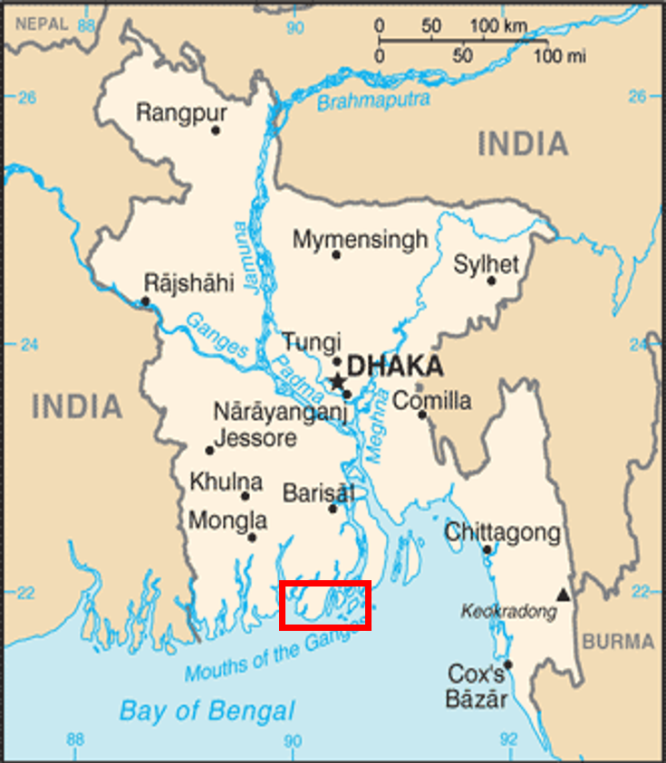
The 338992.8 ha study area is at the east of Barisal River delta (BRD), south-central Bangladesh, shown in figure 1. Barisal is covered by complex mangrove tributary systems from the Brahmaputra-Ganges-Meghna delta. Bangladesh’s coastline has a topographic gradient of 0 to 0.23% (Islam et al, 2019), therefore the low-lying mangroves, are highly vulnerable to rising sea level (Iftekhar and Islam, 2004).
On a global scale, mangrove decline is occurring at a rate of 1- 2% a year, on-track for extinction by the end of the 21st century (Alongi, 2015). In addition, more than 3.6 million ha of mangrove forests were lost from 1980 to 2016 (Asbridge et al, 2016) and many more since. Using NDVI, Saravanan et al (2019) researched 166 ha of mangrove forests from 1999 to 2008 in the Muthupet Lagoon region, South India, retreated due to increased anthropogenic activity India and Bangladesh’s rapid population growth of 43% (Lal, 2020) and 37% (Islam and Ahmed, 2017) over 20 years is a comparable temporal range to this study – meaning it can be expected there will be similar effects on the in the BRD and Muthupet Lagoon region mangrove forests.
Figure 1. Map of Bangladesh (University of Texas Libraries, 2016) showing location of study area indicated by box.
3. Methodology
To define the study area, Landsat-5 Thematic Mapper (TM) imagery from USGS Earth Explorer was obtained using the data shown in table 1. Landsat-5 has a high spatial resolution of 30m pixels. The study area measures a longitudinal distance of 81.171 km (2702 pixels), latitudinal distance of 41.62 km (1394 pixels) and total area of 338992.8 ha.
Table 1. Critical information needed to replicate TM images defined study area abstracted from Landsat-5 imagery in USGS Earth Explorer (USGS, 2020)
| Data Type | Value(s) | ||||
| Date of images | 19/02/1988 | 30/01/2010 | |||
| Path and row | 137 and 045 | ||||
| Cloud cover | <10% | ||||
| Corner coordinates | ULx = 182919
|
ULy = 2446770
|
LRx = 263040
|
LRy = 2404980 |
|
| UTM zone number | WGS 84 | ||||
| Critical change threshold values | Vegetation increase = >25%
|
Vegetation decrease = >27%
|
|||
NDVI is the difference in normalised reflectance between visible red light and NIR (Jensen, 2005) displayed as pixel brightness (Hamylton, 2017). This is determined by the degree of photosynthetically active vegetation, also described as vegetation ‘greenness’ (Wylie et al, 2003). NDVI is calculated using the following equation: NDVI = (NIR – RED) / (NIR + RED). Output values closer to -1 mean there is a lower pixel brightness/little vegetation and values nearer +1 having a high pixel brightness/abundance of vegetation. There is strong absorption of photosynthetically active radiation (PAR) in blue and red visible light and a small solar maximum brightness peak in visible green light where photosynthesising conditions are optimum for healthy vegetation (Lillesand et al, 2015). NDVI was mapped in figure 4 using the threshold values in table 1. From this, amount of increase or decrease can be calculated as a percent of the total area in table 3.
Table 2. Landsat-5 TM spectral band characteristics and main applications for satellite imaging (Pettorelli, 2013) as well as Median pixel brightness Digital Number (DN) for the two images in this study
| Spectral band | Wavelength (µm) | Spectral range | Main applications | Median pixel brightness (DN) |
| Band 1 | 0.45-0.52 | Visible blue | Forest differentiation. | 88 |
| Band 2 | 0.52–0.60 | Visible green | Vegetation reflectance. | 40 |
| Band 3 | 0.63–0.69 | Visible red | Land covers. | 39 |
| Band 4 | 0.76–0.90 | Near infra-red | Eliminates soil moisture. | 26 |
| Band 5 | 1.55–1.75 | Short wave infra-red 1 | Atmospheric penetration. | 13 |
| Band 7 | 2.08–2.35 | Short wave infra-red | Geological use. | 7 |
Table 2 includes brief summaries of spectral bands 1-5 and 7 used in this study to map NDVI. Band 6 is not required as its main application is thermal mapping. The 6 bands are stacked so produce a true-colour image multi-dataset. False-colour images figures 3(a) and 3(b) were created using a multispectral false colour composite: Band 4 (near infra-red (NIR) displayed as red, band 3 (visible red) displayed as green and band 2 (visible green) displayed as blue.
3. Results
Figures 3(a) and 3(b) are NDVI false-colour composite subset images of the Barisal mangroves in 1988 and 2010. The false red colour is vegetation.
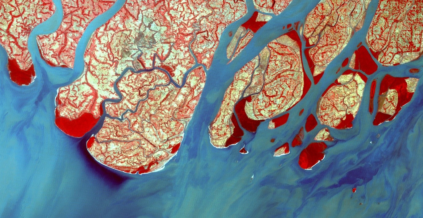
Figure 3(a).1988 false-colour image, 81.17 km wide. False red colour displaying high amounts of vegetation and green and blue showing little vegetation cover. Orientated north to top of image

Figure 3(b). 2010 false-colour image, 81.17 km wide. False red colour displaying high amounts of vegetation and green and blue showing little vegetation cover. Orientated north to top of image
Figure 4 is particularly important for monitoring change in vegetation cover, as it highlights the change of an increase or decrease in vegetation. This is displayed as quantitative data in Table 3, showing change in NDVI as a percentage and in ha. This data will be used as the basis of section 4, discussion.

Figure 4. Change detection NDVI map from 1988 to 2010 superimposed by highlight change map, where green shows areas where NDVI increased >25% and red shows areas where NDVI has decreased >27%. White box highlights area of high mangrove decrease. Image 81.17 km wide, orientated north to top of image
Table 3. Quantitative data from figure 4 to show NDVI change in area (ha to 1 DP) and as a percentage of total area (% to 2 DP)
| Significant decrease | Insignificant change | Significant increase | Total area | |
| Area (ha) | 9472.7 | 319222.9 | 10297.2 | 338992.8 |
| Percentage of total area (%) | 2.79 | 94.17 | 3.04 | 100 |
4. Discussion
In Table 3, 2.79% of the total study area experienced a decrease in mangrove cover across the BRD between 1988 and 2010. 3.04% of the study area does not support this and instead shows an increase in mangrove cover. However, there is only a 0.25% net increase, meaning the possible causes of these changes must be analysed on a specific area scale as the change is not significant enough to make an overall judgement.
Significant decrease in mangrove cover applies greatly to the area of the white box on figure 4 because there is a net decrease of 15.3% (35.0% of overall decrease). As introduced, anthropogenic global warming and the effects on ecosystem supporting services contribute to mangrove decrease in Bangladesh. Over the last century, global sea level has risen around 2 mm, with one half of this due to thermal expansion – the increased volume of oceans due to addition of melted ice (Dyurgerov, Meier, 1997). Sea level rise in the Bengal delta undoubtedly exceeds the global mean, being sometimes as high as 25 mm per year (Ericson et al, 2006).
Bangladesh’s high topographic coastline means a 25 mm sea level rise is likely to submerge the low-lying mangroves, hence the decreases in mangrove cover across the study area. On top of this, submergence of mangroves is exacerbated by urban and agricultural expanse (Saintilan et al, 2014) because a physical barrier is created to prevent mangroves ‘back stepping’ inland. Figures 6(a) and 6(b) suggest evidence of these barriers by contrasting false-colour composites.
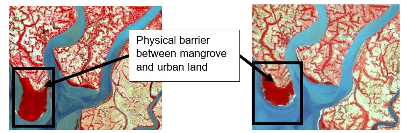
Figures 6(a) and 6(b). 1988 (6a) and 2010 (6b) false-colour composite images, 20734.5 km across, cropped from the study area. Shows labelled physical barrier in highlighted black box. Orientated north to top of image
Dam creation, irrigation and deforestation alter supporting ecosystem services, affect the BRD mangroves. Diverting fresh surface waters for irrigation increases saline water levels in the river delta by moving the saline interface inland (Sahagian, 2000). If salinity is too high, mangrove productivity falls as excessive filtering is too energetically expensive (Santini, 2015).
Coastal protection of mangroves may explain the 3.04% significant increase in NDVI. 39.4% of Barisal’s population is at the upper poverty line, compared to a country average of 31.5% (World Bank, 2010). Researchers like Dasgupta et al (2019), Loughland et al (2020) and Hu et al (2020) have realised the benefits mangrove protection and afforestation has for climate mitigation as well as socio-economics in Bangladesh. In turn, deprived regions like Barisal will benefit as agricultural land is less likely to be flooded -increasing crop yields (this extent of success can be measured by NDVI).
Another driving factor for mitigation is to increase biodiversity. In Kuwait, Loughland et al (2020) studied a mangrove planting scheme with growth success up to 62% of which 57% is in the intertidal zone, prone to climatic flooding (Al-Nafisi et al, 2009). Hu et al (2020) used a restoration potential index (RPI) to conclude that across China, 16,800 ha of land had mangrove restoration capacity. However, 75% of this area became unsuitable for restoration, proving the short-term volatility of mangroves. Nevertheless, if the increase in mangrove cover across the BRD is due to afforestation, it could be questioned why the whole Barisal study area was not protected, since there are larger mitigation schemes in other cases.
NDVI imaging like figure 4 can be used to design planning strategies for Non-Governmental Organisations, charities and private sectors with an aim to restore mangrove forests. Additionally, mapping NDVI matters strongly in the context of climate change. The Intergovernmental Panel on Climate Change estimated an average global sea level rise of 30 to 60 cm by 2100, due to emissions promoting warming by 15 to 78% over the next century (IPCC, 2019). In order to plan mitigation strategies, evidence for mangrove destruction is useful publication for proving the effects of climate change; NDVI monitors change overtime, therefore this is an ideal tool for this. Subsequently, comparisons can be made using NDVI data, such as to crop yields.
Satellite imagery of NDVI poses some drawbacks which have been considered for this study. It is essential when measuring vegetation change on a large temporal scale (not seasonally), the images must be from the same (±1) month. This avoids seasonal differences, such as leaf cover and cyclones, which may produce inaccurate annual NDVI values. Soil moisture can distort values as wetter soil is darker, so NDVI can appear to change as a result of seasonal soil moisture changes and not because of vegetation cover (Pettorelli, 2013). In figure 4, insignificant vegetation change is disregarded due to small-scale variations or no change at all.
Cloud cover can create shadows and scattering (radiating waves change direction of travel when contacting particles and molecules in the atmosphere), leading to possible inaccurate NDVI values as pixel brightness can reduce (Tanre et al, 1992). Cloud cover is thick in tropical regions, therefore <10% cloud cover is needed when mapping Bangladesh. Striping is a remote-sensing anomaly where visible lines appear on the image for a number of reasons, but particularly internal calibration problems of sensors for Landsat Multispectral Scanner imaging (Tsai and Chen, 2008). Striping is visible on figure 6, though has no serious implication on the image. In addition to the high spatial resolution of Landsat-5, the shallow topography of the study area improves NDVI accuracy as few shadows are created from physical and man-made structures on the surface. Therefore, if the images are taken from an oblique angle, shadowing is less likely to influence NDVI values (Thomas, 1997).
5. Conclusions
Since NDVI is a widely used indicator to measure changes in vegetation cover spatially and temporally, it was used to create a false colour composite map of the BRD mangroves in 1988 and 2010. NDVI assessed photosynthetic capacity of vegetation by measuring pixel reflectance at different wavelengths, with healthy, increasing vegetation showing a peak in visible green. Therefore, NDVI was mapped in figure 4 to highlight vegetation areas with a percentage increase or decrease. This data was mapped to accurately observe mangrove cover dynamics as an impact of climate change in the study area from 1988 to 2010.
The study area experienced a 2.79% significant decrease and a 3.04% significant increase in mangrove cover from 1988 to 2010. From scientific literature and similar studies, the significant decrease was likely due anthropogenic activity contributing to global warming (sea level rise and storm surges), irrigation and dam creation thus disrupting supporting ecosystem services. On the other hand, the significant increase is likely due to mangrove restoration schemes. However, net change of the whole study area and local in-the-field research is not significant enough to make definitive judgement on the cause of increase and decrease in mangrove cover. This research can be utilised for showing the effects of anthropogenically-induced climate change on mangrove ecosystems in the future.
References
Al-Nafisi, R.S., Al-Ghadban, A., Gharib, I. and Bhat, N.R., 2009. Positive impacts of mangrove plantations on Kuwait’s coastal environment. European Journal of Scientific Research, 26(4), 510-521.
Alongi, D.M., 2015. The impact of climate change on mangrove forests. Current Climate Change Reports, 1(1), 30-39.
Asbridge, E., Lucas, R., Ticehurst, C., Bunting, P., 2016. Mangrove response to environmental change in Australia’s Gulf of Carpentaria. Ecology and evolution, 6(11), 3523-3539.
Dasgupta, S., Islam, M.S., Huq, M., Huque Khan, Z. and Hasib, M.R., 2019. Quantifying the protective capacity of mangroves from storm surges in coastal Bangladesh. PloS one, 14(3).
Dyurgerov, M. B. and Meier, M. E., 1997. Year-to-year fluctuations of global mass balance of small glaciers and their contributions to sea-level changes, Arct. Alp. Res, 29(4), 392-402.
Ericson, J.P., Vörösmarty, C.J., Dingman, S.L., Ward, L.G. and Meybeck, M., 2006. Effective sea-level rise and deltas: Causes of change and human dimension implications. Global and Planetary Change, 50(1-2), 63-82.
Hamylton, S. M., 2017. Spatial analysis of coastal environments. Cambridge University Press, 2017, 5, 133.
Hu, W., Wang, Y., Zhang, D., Yu, W., Chen, G., Xie, T., Liu, Z., Ma, Z., Du, J., Chao, B. and Lei, G., 2020. Mapping the potential of mangrove forest restoration based on species distribution models: A case study in China. Science of The Total Environment, 748, 142321.
Iftekhar, M.S. and Islam, M.R., 2004. Managing mangroves in Bangladesh: A strategy analysis. Journal of Coastal Conservation, 10(1), 139-146.
IPCC., 2019. Summary for Policymakers. In: IPCC Special Report on the Ocean and Cryosphere in a Changing Climate. IPCC.
Islam, M.A. and Ahmed, P., 2017. Prediction of the Population of Bangladesh, Using Logistic Model. International Journal of Applied Mathematics & Statistical Sciences (IJAMSS), 6(6), 37-50.usgs
Islam, M.M., Borgqvist, H. and Kumar, L., 2019. Monitoring Mangrove forest landcover changes in the coastline of Bangladesh from 1976 to 2015. Geocarto International, 34(13), 1458-1476.
Jensen, J.R., 2005. Introductory Digital Image Processing: A Remote Sensing Perspective. 3rd ed. Prentice-Hall Series in Geographic Information Sciences. Upper Saddle River, NJ: Pearson Prentice Hall.
Lal, S., 2020. Mathematical modelling of Population forecasting in India. Interdiscip. Cycle Res, 12(1), 275-283.
Lillesand, T.M., Kiefer, R.W., Chipman, J.W., 2015. Remote sensing and image interpretation. Hoboken, NJ: Wiley, 1, 1-84.
Loughland, R., Butt, S.J. and Nithyanandan, M., 2020. Establishment of mangrove ecosystems on man-made islands in Kuwait: Sustainable outcomes in a challenging and changing environment. Aquatic Botany, 167, 103273.
Morawitz, D.F., Blewett, T.M., Cohen, A. and Alberti, M., 2006. Using NDVI to assess vegetative land cover change in central Puget Sound. Environmental monitoring and assessment, 114(1-3), 85-106.
Pettorelli, N., 2013. The normalized difference vegetation index. Oxford University Press, 1-11.
Quern, C.A.S., Beneditti, C.A., Machado, N.G., da Silva, M.J.G., da Silva Querino, J.K.A., dos Santos Neto, L.A. and Biudes, M.S., 2016. Spatiotemporal NDVI, LAI, albedo, and surface temperature dynamics in the southwest of the Brazilian Amazon forest. Journal of Applied Remote Sensing, 10(2).
Reiche, J., Verbesselt, J., Heckmann, D. and Herold, M., 2015. Fusing Landsat and SAR time series to detect deforestation in the tropics. Remote Sensing of Environment, 156, 276-293.
Sahagian, D., 2000. Global physical effects of anthropogenic hydrological alterations: sea level and water redistribution. Global and Planetary Change, 25(1-2), 39-48.
Saintilan, N., Wilson, N.C., Rogers, K., Rajkaran, A. and Krauss, K.W., 2014. Mangrove expansion and salt marsh decline at mangrove poleward limits. Global change biology, 20(1), 147-157.
Santini, N.S., Reef, R., Lockington, D.A. and Lovelock, C.E., 2015. The use of fresh and saline water sources by the mangrove Avicennia marina. Hydrobiologia, 745(1), 59-68.
Saravanan, R., Jegankumar., Selvaraj, A., Jennifer, J.J. and Parthasarathy, K.S.S., 2019. Utility of Landsat Data for Assessing Mangrove Degradation in Muthupet Lagoon, South India. Elsevier. 20, 471-484.
Tanre, D., Holben, B.N. and Kaufman, Y.J., 1992. Atmospheric correction algorithm for NOAA-AVHRR products: theory and application. IEEE Transactions on Geoscience and Remote Sensing, 30(2), 231-248.
Thomas, W., 1997. A three-dimensional model for calculating reflection functions of inhomogeneous and orographically structured natural landscapes. Remote sensing of environment, 59(1), 44-63.
Tsai, F. and Chen, W.W., 2008. Striping noise detection and correction of remote sensing images. IEEE Transactions on Geoscience and remote sensing, 46(12), 4122-4131.
USGS, 2020. Earth Explorer. [online] available at: https://earthexplorer.usgs.gov/ (accessed 17/10/20).
World Bank., 2010. [Online] Bangladesh poverty map 2010-technical report. Dhaka: World Bank, Bangladesh Bureau of Statistics, and World Food Programme; 2014a. Available at: http://www-wds.worldbank.org/external/default/WDSContentServer/WDSP/IB/2014/11/11/000442464_20141111221335/Rendered/PDF/904870v20Bangl0LIC000Sept004020140.pdf (accessed 2/12/20).
Wylie, B.K., Johnson, D.A. Laca, E., Saliendra, N.Z., Gilmanov, T.G., Reed, B.C., Tieszen, L.L. and Worstell. B.B., 2003. Calibration of Remotely Sensed, Coarse Resolution NDVI to CO2 Fluxes in a Sagebrush-Steppe Ecosystem. Remote Sensing of Environment, 85(2), 243–255.


#Data source


Next article

The field of Earth observation and applications for EO data are expanding rapidly. However, developers and data scientists who possess the next big idea for using EO data often face a major roadblock: limited funds and resources. Luckily, the 2021 Copernicus Masters Challenges are here to support tech-savvy innovators as they bring their ideas to life. Copernicus Masters is a set of global challenges asking participants to use EO data to improve and preserve daily life. Through the challenges, participants compete for prizes to back their work such as free data and cash winnings.
UP42, a global provider of geospatial data through its platform and marketplace, is offering a Copernicus Masters challenge as one of the program’s partners. The company is calling on researchers, companies, and students to develop an image augmentation algorithm to address common issues hindering EO analytics.
To qualify, these algorithms must use generative adversarial networks (GANs)—an innovative deep learning approach that is becoming an industry standard for its ability to produce higher-resolution imagery from low-resolution data input.
Participants will focus their algorithm on solving one of three issues:
- Unsupervised change detection—GANs can be used to generate better coregistered images via synthetic image generation.
- Clouds and shadows in optical satellite imagery—these obstacles affect almost all land, water, and atmosphere applications.
- Super-resolution satellite imagery—increasing the resolution can widen the range of objects detected from a given data set.
To develop an algorithm, participants will have access to very-high-resolution imagery from UP42’s content partner Airbus and data from all Sentinel missions via the sobloo platform.
UP42 chose to offer this challenge because it ties in with the company’s core mission of democratizing access to Earth insights. By offering access to data and the tools to innovate with Earth observation, the company hopes to inspire more change-makers to think beyond what’s currently being done in the industry to solve real-world challenges like climate change and food insecurity.
Winner Takes All for UP42 Copernicus Masters Challenge
To determine the challenge winner, projects will be judged on four criteria: scientific value, product and business value, quality of implementation, and ecological impact.
The winner of the UP42 challenge will receive three rewards to support their work:
- OneAtlas Prize: a voucher to access commercial satellite data from Airbus
- UP42 Prize: a voucher to access geospatial data and algorithms from the UP42 marketplace
- Satellite Data: up to EUR 10,000 worth of commercial datasets from the Copernicus Contributing Missions
Copernicus Masters will also have an overall winner who will take home a EUR 10,000 prize—a solid investment for turning their project into a full-fledged business.
To compete for these prizes, be sure to register, choose the UP42 partner challenge, and enter your project details into the secure database by 19 July 2021. Submissions will be evaluated by October, and challenge finalists will be notified by November. In December, an awards ceremony will recognize the Copernicus Masters winner.
Need a little inspiration before starting your project? Check out the past winners’ Hall of Fame to see what’s possible in the Copernicus Masters Challenges.